The single equation that changed NLP shipped in 2017 inside Attention Is All You Need (Vaswani et al.). Scaled dot-product self-attention replaced recurrence, convolution, and alignment models with one operation. Every LLM since, from GPT to DeepSeek, runs on variants of it.

By the end of this post you will have built, from scratch in PyTorch, working implementations of Self-Attention, Multi-Head Attention, Causal Self-Attention, and Cross-Attention, the four building blocks that power every transformer.

No history lesson. No survey of 200 papers. Just the mechanics, the shapes, and the code. If you know what a tensor is and can read a nn.Module, you’re ready.

All code in this post is available as runnable Jupyter notebooks at github.com/david-hoangt/llm_from_scratch.

Note: We’ll thread a single running example through the entire post: the sentence “The CEO announced record earnings on Friday”, embedded into d_model = 64. Watch how each mechanism transforms these vectors step by step.

Self-Attention

Right now, each of our 7 tokens [“The”, “CEO”, “announced”, … “Friday”] is an isolated 64-dimensional vector. “announced” has no idea that “CEO” is its subject or that “Friday” is when it happened. How does a model let every token decide which other tokens matter, without any hardwired positional rules?

Self-attention computes a weighted sum of all other tokens’ representations, with weights determined by learned relevance, not fixed position. This is the atomic operation inside every transformer layer: BERT’s encoder, ViT’s patch interactions, the encoder side of T5. All bidirectional self-attention. Decoder-only models (GPT, LLaMA) use the causal variant we’ll cover later.

Query, Key, and Value

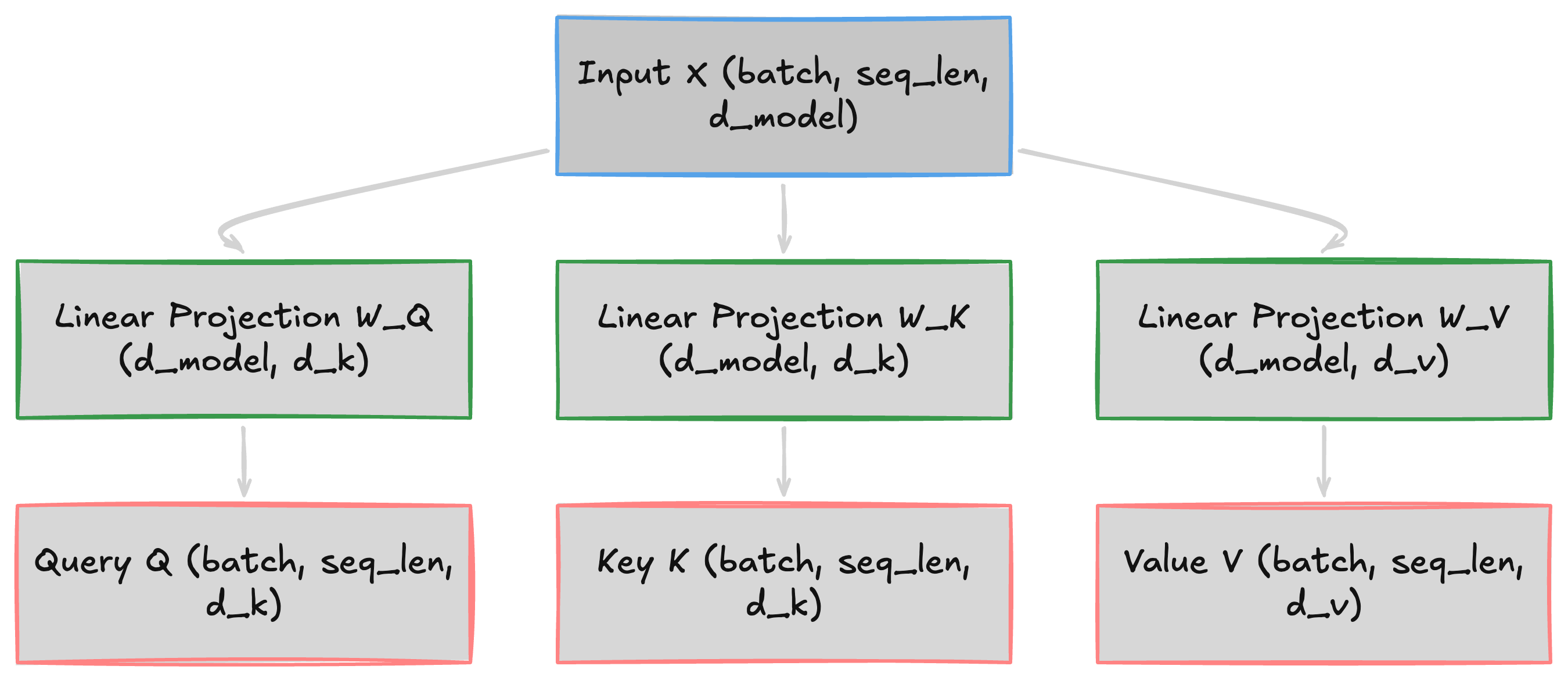
Each token’s embedding is a single vector, but it needs to play three roles at once. “announced” needs to search for its subject, while “CEO” needs to advertise that it is one, and both need to transmit their content when matched. A single vector can’t encode “what am I looking for” and “what do I offer” simultaneously, so we project the input into three separate spaces:

Q = X @ W_Q    K = X @ W_K    V = X @ W_V

• X [batch, seq_len, d_model]: Input embeddings
• W_Q, W_K [d_model, d_k]: Project each token into query and key spaces
• W_V [d_model, d_v]: Project each token into value space
• Q [batch, seq_len, d_k]: What this token is looking for
• K [batch, seq_len, d_k]: What this token advertises
• V [batch, seq_len, d_v]: The content transmitted when attention is paid

Two tokens interact strongly when their query-key dot product is high. “announced” is looking for a subject, and “CEO” advertises exactly that. The diagram below shows this three-way split from a single input embedding:

In practice (and in all implementations below), we set d_v = d_k. The math generalizes to d_v ≠ d_k, but most architectures use equal dimensions for simplicity.

Scaled Dot-Product Attention

Those Q, K, V matrices are ready. “announced” now has a query vector, and “CEO” has a key vector. Their dot product measures how relevant they are to each other. But raw dot products between 64-dimensional vectors produce scores in the hundreds, pushing softmax into near-one-hot regions where gradients vanish. How do you turn them into stable, interpretable weights?

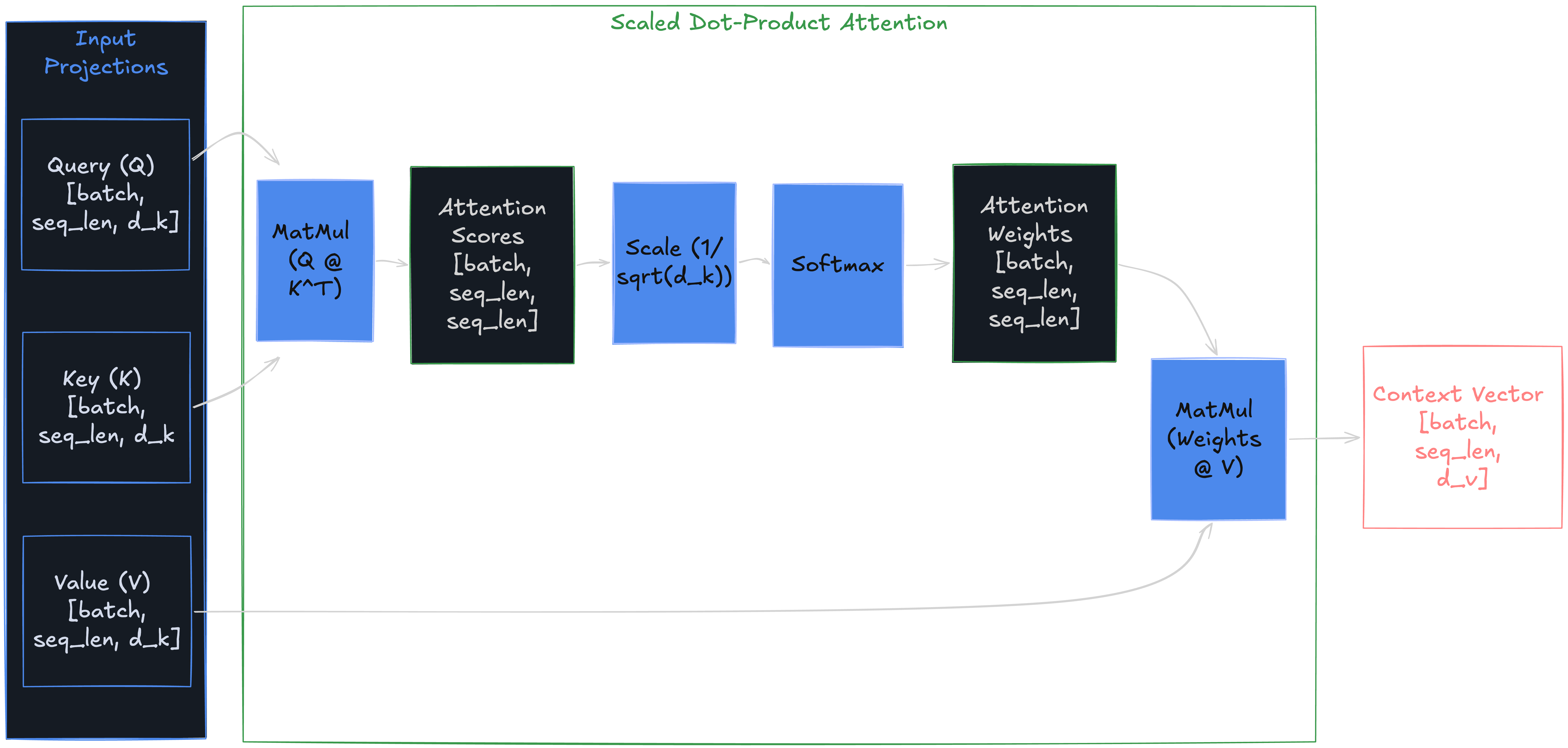
Attention(Q, K, V) = softmax(Q @ K.T / sqrt(d_k)) @ V

• Q @ K.T → [batch, seq_len, seq_len] — Raw relevance scores between all token pairs
• sqrt(d_k) (scalar) — Scaling factor. Dot product variance grows with d_k, saturating softmax
• attn_weights → [batch, seq_len, seq_len] — Row-wise probability distribution
• Output → [batch, seq_len, d_v] — Weighted average of all value vectors

Without scaling, each element in Q @ K.T is a sum of d_k products; variance grows linearly with d_k, pushing softmax into near-one-hot regions where gradients vanish. Divide by sqrt(d_k) to keep the distribution smooth. Multiply by V to produce the final output: each token’s new representation is a weighted mix of all values.

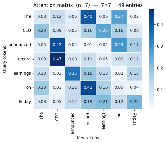
In our 7-token example, the attention matrix is [1, 7, 7]. The row for “announced” peaks on “CEO” (subject) and “earnings” (object).

That’s the full mechanism. Translating it into code is straightforward.

Implementation from Scratch

class SelfAttention(nn.Module):
    def __init__(self, d_model: int, d_k: int | None = None):
        super().__init__()
        self.d_k = d_k if d_k is not None else d_model
        self.W_q = nn.Linear(d_model, self.d_k, bias=False)
        self.W_k = nn.Linear(d_model, self.d_k, bias=False)
        self.W_v = nn.Linear(d_model, self.d_k, bias=False)

    def forward(self, x: torch.Tensor) -> tuple[torch.Tensor, torch.Tensor]:
        Q = self.W_q(x)  # (batch, seq_len, d_k)
        K = self.W_k(x)  # (batch, seq_len, d_k)
        V = self.W_v(x)  # (batch, seq_len, d_k)
        scores = torch.bmm(Q, K.transpose(1, 2)) / math.sqrt(self.d_k)
        weights = F.softmax(scores, dim=-1)  # (batch, seq_len, seq_len)
        out = torch.bmm(weights, V)          # (batch, seq_len, d_k)
        return out, weights

Simple, but expensive. Every token attends to every other token.

📓 Run the full self-attention notebook — includes bidirectional and causal modes with shape checks and attention heatmaps.

Computational Cost

Complexity: O(n² × d) time and memory. A 4,096-token sequence → ~16.8M entries per head per layer. At 128k tokens → ~16.4B. This quadratic scaling motivates every efficiency variant (such as sparse attention, Flash Attention, etc). The chart below shows how the attention matrix grows with sequence length:

Key Takeaways

Self-attention projects each token into Q, K, V spaces, computes scaled dot-product scores, and outputs a weighted combination of all value vectors, making every token’s new representation a function of the entire sequence. It’s the atomic unit of transformer attention, used in every encoder (BERT, ViT, T5 encoder) and as the core of every decoder. Powerful all-to-all connectivity at O(n²) time and memory cost.

A single head can only capture one type of token relationship: “announced” attends to both “CEO” and “Friday” through the same weights. What if different positions need different relationship types?

Multi-Head Attention (MHA)

One head captures one relationship type. What if “announced” needs to attend to “CEO” for subject-verb agreement and to “Friday” for temporal grounding, simultaneously?

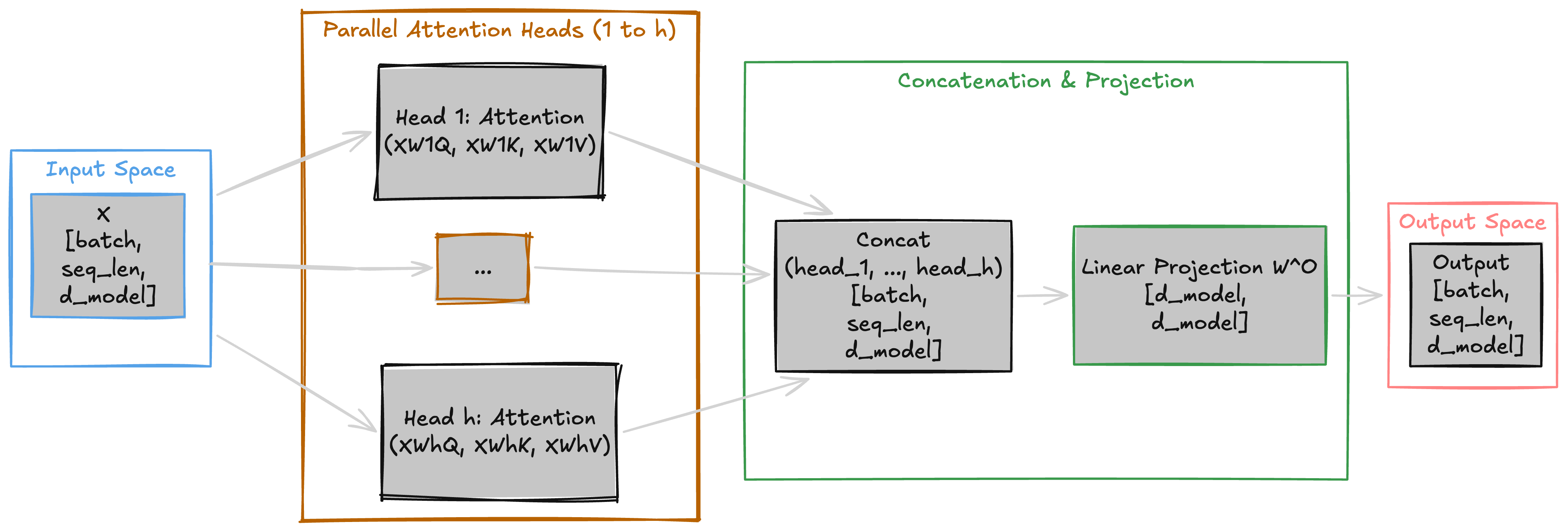
MHA solves this by running h independent heads in parallel, each with its own Q/K/V projections learning different relationship types, then combining their outputs through a learned projection W_O.

The Three-Stage Pipeline

head_i = Attention(X @ W_i_Q,  X @ W_i_K,  X @ W_i_V)
Output = Concat(head_1, ..., head_h) @ W_O

• Stage 1 — Parallel projections: Each head i projects into d_k = d_model / h. With d_model = 64 and h = 4, each head works in 16 dimensions → head_i: [batch, seq_len, d_k]
• Stage 2 — Concatenation: Stack all head outputs along the feature dim → [batch, seq_len, h * d_k] = [batch, seq_len, d_model]
• Stage 3 — Output projection: W_O [d_model, d_model] mixes heads → [batch, seq_len, d_model]

Each head computes scaled dot-product attention in its own d_k-dimensional subspace. One learns subject-verb links (“announced” → “CEO”), another temporal relations (“announced” → “Friday”). W_O mixes these patterns into a unified representation. The diagram below traces data through all three stages:

The Dimension Split

A natural question: doesn’t running h heads cost h times more? No. Each head works in d_k = d_model / h, not full d_model. With d_model = 64 and h = 4: each head is 16-dimensional. Total parameters across all heads ≈ one full-dimensional head. MHA is a better allocation of the same compute budget, not a more expensive one.

The implementation reuses the SelfAttention class from earlier, one instance per head.

Implementation from Scratch

class MultiHeadAttention(nn.Module):
    def __init__(self, d_model: int, n_heads: int):
        super().__init__()
        self.d_k = d_model // n_heads
        self.heads = nn.ModuleList([SelfAttention(d_model, self.d_k) for _ in range(n_heads)])
        self.W_o = nn.Linear(d_model, d_model, bias=False)

    def forward(self, x: torch.Tensor):
        outs, weights = [], []
        for head in self.heads:
            h_out, h_w = head(x)
            outs.append(h_out)
            weights.append(h_w)
        out = self.W_o(torch.cat(outs, dim=-1))   # (batch, seq_len, d_model)
        return out, torch.stack(weights, dim=1)    # weights: (batch, n_heads, seq_len, seq_len)

📓 Run the multi-head attention notebook — includes per-head visualizations and a detailed single-head vs. multi-head comparison table.

Key Takeaways

h parallel heads in d_model / h subspaces, combined via learned W_O, with the same total compute as single-head. MHA is the original design (GPT-2, OLMo); newer models use GQA (Llama 3) or MLA (DeepSeek V3) to reduce KV cache cost.

MHA gives every head full access to all positions, but for autoregressive generation, “Friday” shouldn’t peek at tokens that come after it. One additive mask solves this.

Causal Self-Attention

Standard attention lets every token see every other token, including the future. When the model is trying to predict what comes after “The CEO announced”, position 3 can look ahead and see “record” sitting at position 4. It just copies instead of learning to predict. That’s where causal masks come in.

CausalAttention(Q, K, V) = softmax(Q @ K.T / sqrt(d_k) + M) @ V

Add one hard constraint to standard attention: each token sees only itself and earlier positions. This is the attention mechanism inside every decoder-only LLM — GPT, Claude, LLaMA, Mistral — where the model generates one token at a time, left to right. Without this mask, the model copies instead of predicts.

The Mask Mechanism

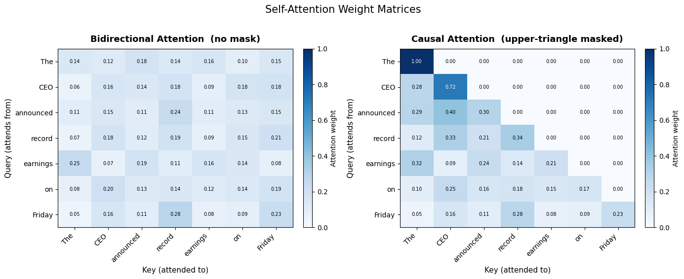
We need position 3 (“announced”) to attend only to positions 0–3, while position 6 (“Friday”) can see everything. Add −∞ to the banned positions before softmax. They get exactly zero weight:

M[i][j] = 0       if j <= i
M[i][j] = -inf    if j > i

• Mask added before softmax, to scaled scores
• Effect of e^−∞: exactly zero attention weight
• Result: lower-triangular attention matrix
• Reuse: computed once, shared across all heads and layers
• Training: all T positions computed in one forward pass. Position t sees tokens 0…t simultaneously, no T separate passes needed

Add M to Q @ K.T / sqrt(d_k) before softmax. Future positions get -inf, softmax maps them to exactly zero. The mask is built with torch.triu(..., diagonal=1) which produces the upper-triangular boolean, and masked_fill sets those positions to -inf.

In our 7-token example, “CEO” (position 1, 0-indexed) sees only [“The”, “CEO”]. “Friday” (position 6) sees the full sequence. The attention matrix is lower-triangular: 28 active entries out of 49.

Concretely: when generating “The CEO announced ___”, position 3 attends only to [“The”, “CEO”, “announced”]. It cannot see “record” at position 4 or “Friday” at position 6. If position 3 could peek at position 5, it would just copy “earnings” instead of learning to predict it.

The mask handles training and shapes. But at inference time, the causal constraint unlocks a major optimization.

KV Cache and Inference Cost

The causal mask means token t never attends beyond t, so keys and values for positions 1...t-1 are fixed once computed. Caching them is safe. Bidirectional attention would invalidate the cache with every new token.

During autoregressive generation, each new token attends to all previous tokens. The KV cache stores past key/value tensors to avoid recomputation:

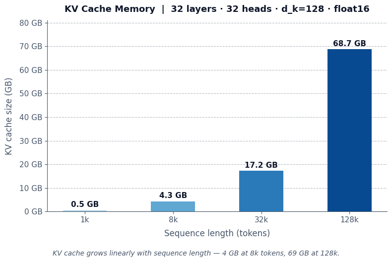
KV cache memory (bytes) = 2 * n_layers * n_heads * T * d_k * bytes_per_element

• 2 = one tensor for K, one tensor for V
• LLaMA 3 8B (32 layers, 32 heads, d_k = 128, T = 8,192) → ~4 GB (float16)
• Same config, T = 128k → ~69 GB (float16)

This linear-in-T memory scaling is the dominant inference bottleneck. It’s why long conversations slow down and why providers charge per-token. It drives GQA (share K/V across head groups) and MLA (compress K/V into a low-rank latent). The chart below shows KV cache memory scaling with sequence length:

Gotcha: many heads assign disproportionate weight to the first token. Under the causal mask, it’s the only position visible to all others, acting as a default “sink” for leftover attention mass (see StreamingLLM).

Implementation from Scratch

class CausalSelfAttention(nn.Module):
    def __init__(self, d_model: int, d_k: int):
        super().__init__()
        self.d_k = d_k
        self.W_q = nn.Linear(d_model, d_k, bias=False)
        self.W_k = nn.Linear(d_model, d_k, bias=False)
        self.W_v = nn.Linear(d_model, d_k, bias=False)

    def forward(self, x: torch.Tensor) -> torch.Tensor:
        Q, K, V  = self.W_q(x), self.W_k(x), self.W_v(x)
        seq_len  = x.size(1)
        scores   = torch.bmm(Q, K.transpose(1, 2)) / math.sqrt(self.d_k)
        mask     = torch.triu(torch.ones(seq_len, seq_len, dtype=torch.bool), diagonal=1)
        weights  = F.softmax(scores.masked_fill(mask, float("-inf")), dim=-1)
        return torch.bmm(weights, V)

📓 Causal attention is covered in the self-attention notebook — the unified SelfAttention class handles both bidirectional and causal modes via an optional mask parameter.

Key Takeaways

Lower-triangular mask enables autoregressive generation, KV caching, and single-pass training, the foundation of every decoder-only model (GPT, LLaMA, Mistral). Bidirectional models (BERT) see everything but can’t generate; encoder-decoder models (T5) combine both via cross-attention.

Causal attention lets a sequence attend to itself with temporal constraints. But what about attending to a completely different sequence?

Cross-Attention

Causal self-attention connects tokens within one sequence. But what if the decoder needs to ask: “which of the encoder’s tokens matter for what I’m generating right now?”

CrossAttention(Q, K, V) = softmax(Q @ K.T / sqrt(d_k)) @ V

Cross-attention connects two separate sequences: queries from one, keys/values from the other. Same formula as self-attention, but Q and K/V come from different sources.

The Mechanism

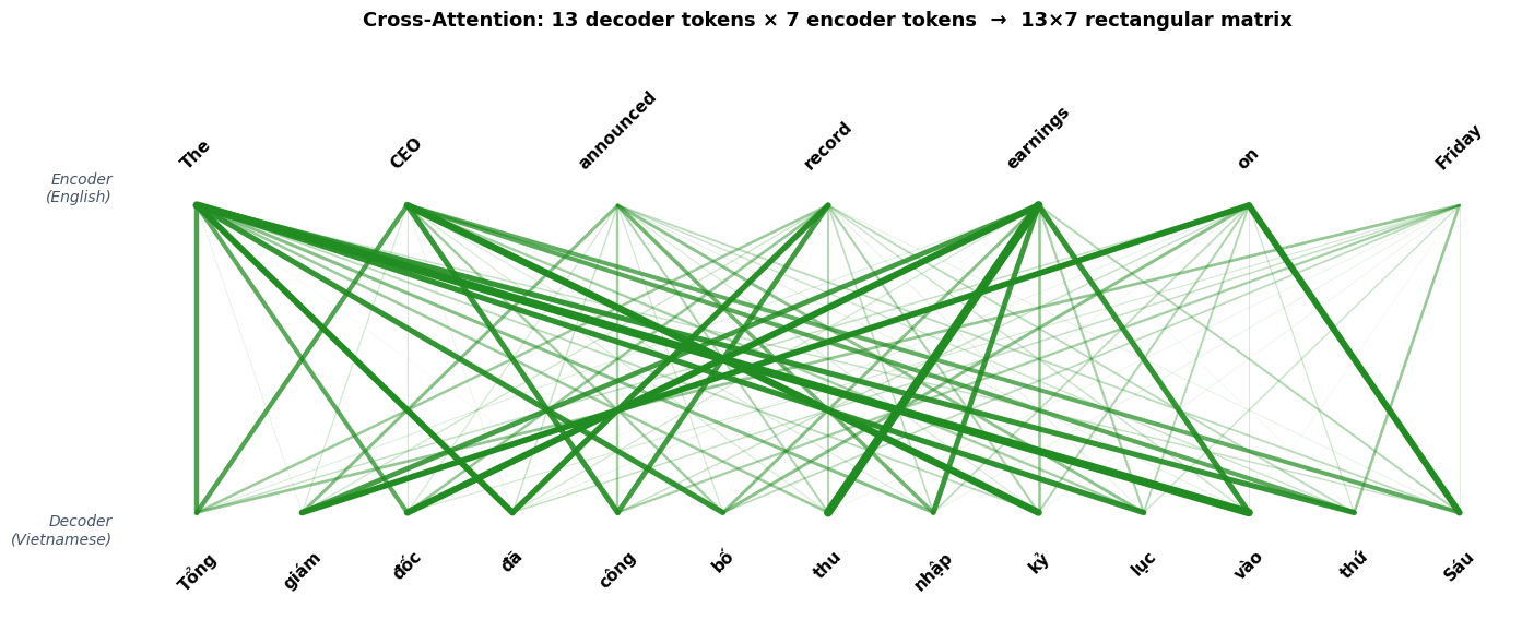
Consider translating “The CEO announced record earnings on Friday” (7 tokens) into Vietnamese: “Tổng giám đốc đã công bố thu nhập kỷ lục vào thứ Sáu” (13 tokens). The decoder generates the Vietnamese output token by token, and at each step it needs to look back at the English source to decide what to translate next. The two sequences have different lengths: 13 Vietnamese tokens querying 7 English tokens.

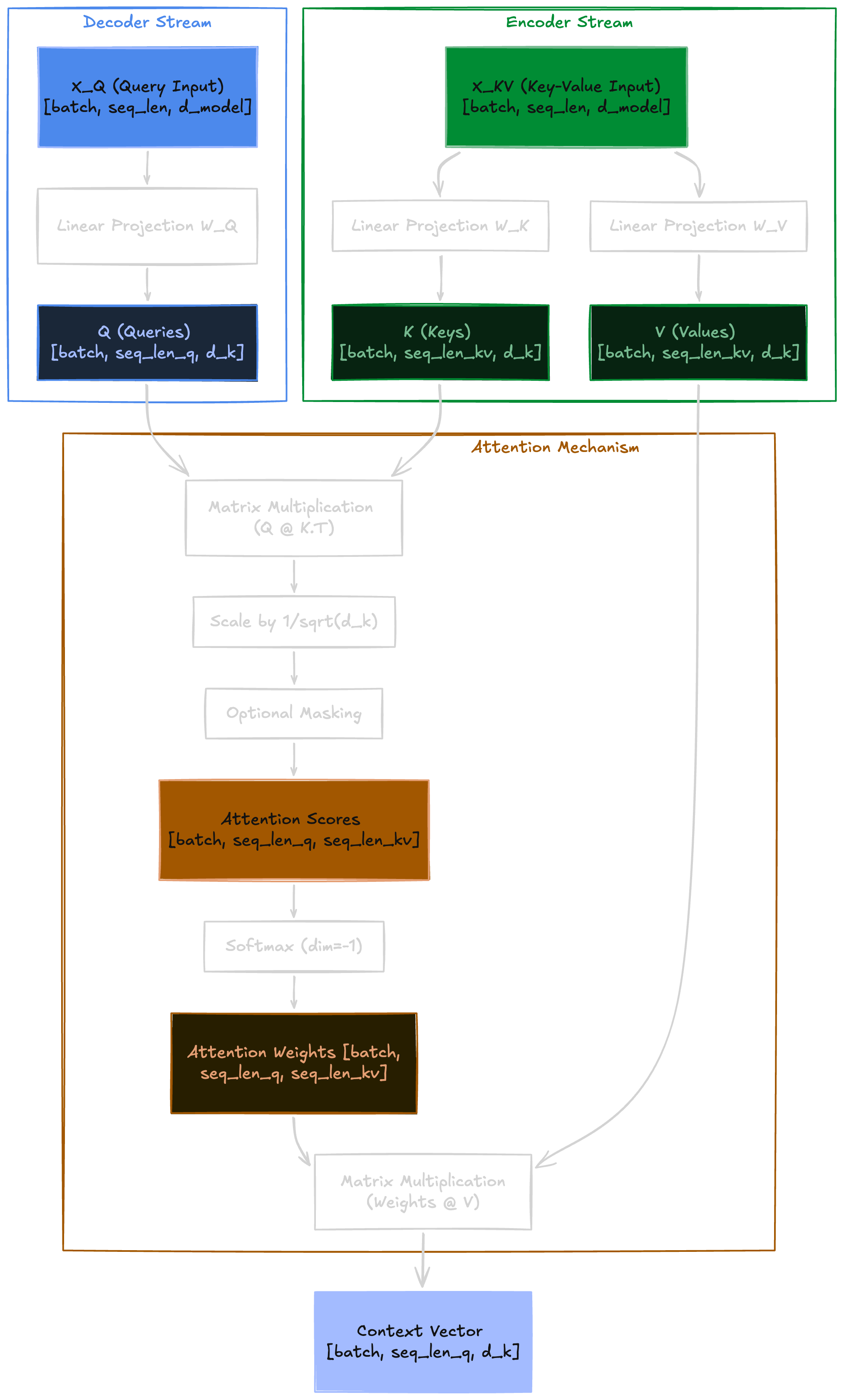
The wiring: Q from one sequence, K/V from the other:

Q = X_Q  @ W_Q       # from decoder: [batch, seq_len_q, d_model] -> [batch, seq_len_q, d_k]
K = X_KV @ W_K       # from encoder: [batch, seq_len_kv, d_model] -> [batch, seq_len_kv, d_k]
V = X_KV @ W_V       # from encoder: [batch, seq_len_kv, d_model] -> [batch, seq_len_kv, d_k]

• X_Q [batch, seq_len_q, d_model] — Querying sequence (decoder)
• X_KV [batch, seq_len_kv, d_model] — Context sequence (encoder)
• Attention matrix [batch, seq_len_q, seq_len_kv] — Rectangular, not square

In our example, the attention matrix is 13 x 7: each of the 13 decoder rows specifies how one Vietnamese token distributes attention across all 7 English tokens.

That covers the mechanism. But cross-attention doesn’t exist in isolation; it’s one of three sub-layers inside each decoder block.

Role in the Original Transformer

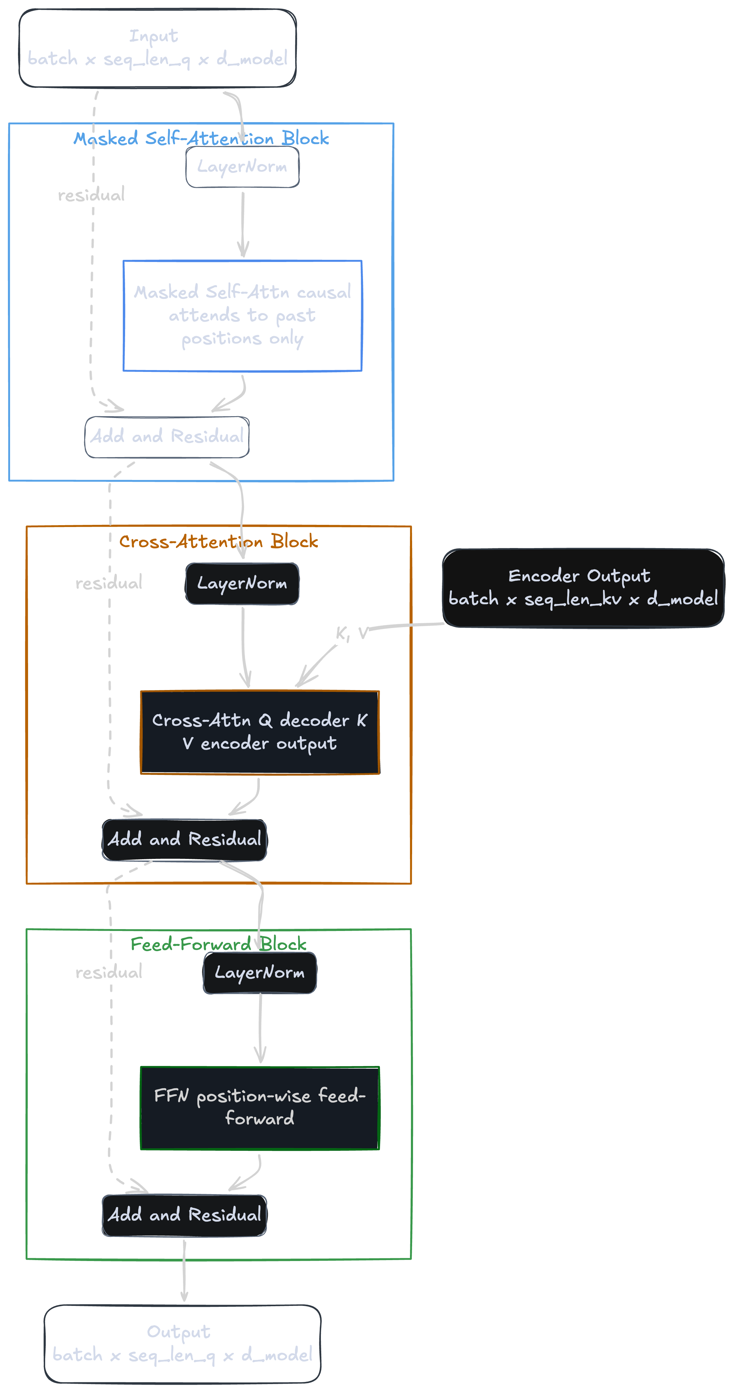
Each decoder block in the original Transformer stacks three sub-layers in sequence:

1. Causal self-attention — Q from decoder, K/V from decoder
2. Cross-attention — Q from decoder, K/V from encoder
3. Feed-forward network — position-wise, no attention

The encoder output is computed once and reused by every decoder layer at every generation step. The diagram below shows the full decoder block with all three sub-layers, residual connections, and the encoder output feeding K/V into the cross-attention layer:

This encoder-decoder design powered the original Transformer. But most modern text-only LLMs have moved away from it entirely.

Cross-Attention vs. Concatenation

Modern text-only LLMs (GPT, LLaMA) are decoder-only — no encoder, no cross-attention. They concatenate the two sequences and let causal self-attention handle the rest. The tradeoff:

• Concatenation — Simpler, no extra architecture. But cost is O((seq_q + seq_kv)²), the combined length quadratic.
• Cross-attention — Cost is O(seq_q × seq_kv), keeping the two sequences separate. But requires dedicated Q/K/V projections wired across encoder and decoder.

For text-only LLMs, concatenation wins. Cross-attention remains dominant in multimodal architectures where the two modalities have very different representations: Flamingo (language → image features), Stable Diffusion (U-Net ← CLIP text), Whisper (decoder ← audio encoder).

Implementation from Scratch

The data flow diagram below maps directly to the code: X_Q feeds W_Q on the decoder side, X_KV feeds W_K and W_V on the encoder side, and both streams merge at the attention computation. Notice that seq_len_q and seq_len_kv are independent — 13 and 7 in our translation example — producing the rectangular matrix from earlier.

class CrossAttention(nn.Module):
    def __init__(self, d_model: int, d_k: int | None = None):
        super().__init__()
        self.d_k = d_k if d_k is not None else d_model
        self.W_q = nn.Linear(d_model, self.d_k, bias=False)
        self.W_k = nn.Linear(d_model, self.d_k, bias=False)
        self.W_v = nn.Linear(d_model, self.d_k, bias=False)

    def forward(self, x_q: torch.Tensor, x_kv: torch.Tensor) -> tuple[torch.Tensor, torch.Tensor]:
        Q = self.W_q(x_q)    # (batch, seq_len_q,  d_k)
        K = self.W_k(x_kv)   # (batch, seq_len_kv, d_k)
        V = self.W_v(x_kv)   # (batch, seq_len_kv, d_k)
        scores = torch.bmm(Q, K.transpose(1, 2)) / math.sqrt(self.d_k)  # (batch, seq_len_q, seq_len_kv)
        weights = F.softmax(scores, dim=-1)  # (batch, seq_len_q, seq_len_kv)
        out = torch.bmm(weights, V)          # (batch, seq_len_q, d_k)
        return out, weights

📓 Run the cross-attention notebook — includes padding mask handling and a translation alignment visualization.

Key Takeaways

Same formula as self-attention, but Q from one sequence and K/V from another → rectangular seq_len_q x seq_len_kv matrix. Bridges encoder-decoder in the original Transformer. Standard for multimodal; replaced by concatenation in text-only LLMs.

Conclusion

Four mechanisms, one core operation. Self-attention gives every token all-to-all connectivity through Q, K, V projections and scaled dot-product scoring. Multi-head attention runs h independent heads in parallel subspaces, then recombines via W_O, with the same compute budget but richer representations. Causal self-attention adds a lower-triangular mask that blocks future positions, enabling autoregressive generation and KV caching. Cross-attention splits Q and K/V across two sequences, producing a rectangular attention matrix that bridges encoder and decoder.

Every transformer since 2017 (GPT, BERT, LLaMA, Whisper, Stable Diffusion) is built from combinations of these four building blocks.

The shapes, the scaling, and the masks are the same; only the wiring changes.